38 excel pivot table conditional formatting row labels

How to Highlight A row based on Cell Value In Pivot Table By selecting the pivot table, the user must point to the 'Home Tab' and must click on the 'Conditional Formatting' menu. From the ' Conditional Formatting ' menu, the user must click on ' New Rules'. When the ' New Formatting Rule Dialogue Box ' opens, the user should select ' use a formula to determine which cells to format ' under the rule types. Pivot Table Conditional Formatting for Different Rows Items? Select Your Pivot Table and: Go to Conditional Formatting -> New Rule -> Choose All cells showing "duration" values for "Type and "Date Selection" under "Apply Rule To" section -> Use a Formula to Determine which cells to format and enter the following formula: =AND (A6="Cars",A6>3), You can create new rules for other two conditions as well:

Excel Conditional Formatting in Pivot Table - EDUCBA Click on any cell in the pivot table > Go to the HOME tab > Click on Conditional Formatting option under Styles option > Click on Manage Rules option. It will open a Rules Manager dialog box. Click on the Edit Rule tab, as shown in the below screenshot. It will open the Editing Rule formatting window. Refer to the below screenshot.

Excel pivot table conditional formatting row labels

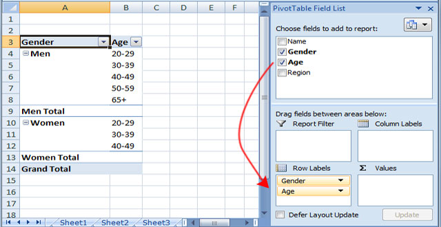
Pivot Table Conditional Formatting Weekend Data Highlight Add Conditional Formatting Follow these steps to apply the weekend highlighting in the pivot table: Select all cells where conditional formatting should be applied, cells B5 to B20 in this example. On the Excel Ribbon, click the Home tab Click Conditional Formatting, and in the drop down menu, click New Rule The New Formatting Rule dialog box opens Conditional Formatting on Pivot Table row labels As per my knowledge, in this case it does not matter what is the source of pivot as after getting the data in pivot, it's the pivot where the conditional formatting need to be applied, please upload a sample. thanks. Regards, DILIPandey DILIPandey +91 9810929744 dilipandey@gmail.com Register To Reply How to make row labels on same line in pivot table? As we all know, the pivot table has several layout form, the tabular form may help us to put the row labels next to each other. Please do as follows: 1. Click any cell in your pivot table, and the PivotTable Tools tab will be displayed. 2. Under the PivotTable Tools tab, click Design > Report Layout > Show in Tabular Form, see screenshot: 3.

Excel pivot table conditional formatting row labels. Highlight Cell Rules based on text labels - MyExcelOnline This is our current Pivot Table setup. We want to highlight all of the Q1 text in our Row Labels. STEP 1: Highlight all the quarter text by clicking above the cell STEP 2: Go to Home > Conditional Formatting > Highlight Cells Rules > Text that Contains STEP 3: Type in Q1 and select OK. You can select any color that you wish. How to rename group or row labels in Excel PivotTable? To rename Row Labels, you need to go to the Active Field textbox. 1. Click at the PivotTable, then click Analyze tab and go to the Active Field textbox. 2. Now in the Active Field textbox, the active field name is displayed, you can change it in the textbox. You can change other Row Labels name by clicking the relative fields in the PivotTable ... How to Apply Conditional Formatting to Pivot Tables - Excel Campus So in this post I explain how to apply conditional formatting for pivot tables. 1. Select a cell in the Values area The first step is to select a cell in the Values area of the pivot table. If your pivot table has multiple fields in the Values area, select a cell for the field you want to apply the formatting to. 2. Apply Conditional Formatting Pivot Table Conditional Formatting with VBA - Peltier Tech sub formatpt2 () dim c as range with activesheet.pivottables ("pivottable2") ' reset default formatting with .tablerange1 .font.bold = false .interior.colorindex = 0 end with ' apply formatting to each row if condition is met for each c in .pivotfields ("category 3").pivotitems ("a").datarange.cells if c.value >= 7 then with …

Pivot Table Conditional Formatting - Computer Tutoring How to Conditionally Format an Entire Row in a Pivot Table? · First select Cell E6. · Then click Conditional Formatting - New Rule. · After that select Use a ... Conditional Formatting in Pivot Table - WallStreetMojo First, let us insert a pivot table in this data. Step 1: We must select the data. Then, in the "Insert" Tab, click on "Pivot Tables." Step 2: Then, insert the pivot table in a new worksheet by clicking "OK." Step 3: Drag down the "Product" in the "Row" label and "Months" in the "Value" fields. The pivot table will look as shown below. conditional formatting per row on pivot - Microsoft Tech Community conditional formatting per row on pivot. I would like to format each row of a pivot table separately (as in the picture shown below), but I cannot paste the formatting. I've got many rows, and they could change (just like the columns) Is there a way to automate this, or I have to select row by row and apply the formatting? Apply Conditional Formatting | Excel Pivot Table Tutorial Go to Home Tab → Styles → Conditional Formatting → New Rule. From rule to, select the third option. And, from "select a rule" type select "Format only top or bottom" ranked values. In edit rule description, enter 1 in the input box and from the drop-down menu select "each Column Group". Apply formatting you want. Click OK.

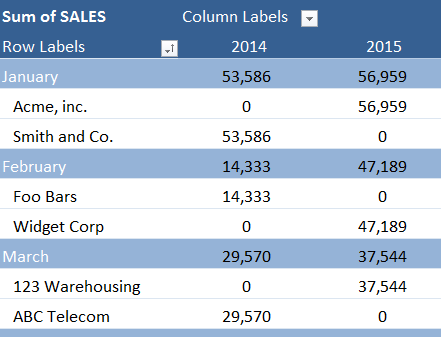
Pivot table conditional formatting - Exceljet Select any cell in the data you wish to format and then choose "New rule" from the conditional formatting menu on the Home tab of the ribbon. At the top of the window, you will see setting for which cells to apply conditional formatting to. For the example shown, we want: "All cells showing sum of "sales values" for name and "date" How to apply conditional formatting to Pivot Tables Go to HOME > Conditional Formatting > New Rule to add a new formatting rule, or select from predefined options. If you select the latter, you will need to configure the rule regardless. The New (or Edit) Formatting Rule window contains options specific to Pivot Tables. You can choose the location where you want to apply your conditional ... Conditional formatting for Pivot Tables in Excel 2016 - 2007 The format I used was to select Conditional Formatting > Top 10 Items > set it to 1 item and select the default format. This format can be copied from one range to the next if desired or built up for each range individually. To copy the format, select one or more cells with that format and click Copy. Conditional Format Pivot Table Row - Chandoo.org Select the entire row, and when you apply the conditional format, make the column reference absolute. So, say we want the entire row 2 to be formatted if cell in col B = 5. formula would be: =$B2=5

Lesson 54: Pivot Table Row Labels - Swotster

How to Apply Conditional Formatting to Rows Based on ... - Excel Campus On the Home tab of the Ribbon, select the Conditional Formatting drop-down and click on Manage Rules…. That will bring up the Conditional Formatting Rules Manager window. Click on New Rule. This will open the New Formatting Rule window. Under Select a Rule Type, choose Use a formula to determine which cells to format.

√ダウンロード change table name excel 365 255677-Office 365 excel change table name

Pivot Table Conditional Formatting - Microsoft Tech Community Hi all :) I have an issue conditionally formatting a Pivot Table. I have my row hierarchy set up as Region, Area, Store, Consultant. My rows are expanded out only to a Store Level. I need the Store Name to be highlighted red if the value in the first column is <1. I have applied conditional fo...

vba - Pivot Table with Conditional Formatting: Where did my indents go? - Stack Overflow

In a pivot table, how to apply conditional formatting by label ... 1 Answer 1 ... You select the item you want to apply the formatting to, then create the rule. With your pivot table, if you hover over the left- ...

How to Create a MS Excel Pivot Table – An Introduction | SIMPLE TAX INDIA

Excel VBA: Conditional Format of Pivot Table based on Column Label then by creating a pivot table, you will have these items: Cola, Fanta, 'Sum of Price', and the following field labels: 'Row labels', 'Sum of Price'. If you try to use 'Sum of Price' in the PivotTable.PivotSelect function, then the error message in the question will appear.

How to Insert a Blank Row in Excel Pivot Table | MyExcelOnline

Excel Gantt Chart with Conditional Formatting (2 Examples) Now, we have to apply the general conditional formatting like the previous example. For that, select the range of cells G5:U9. After that, in the Home tab, click on the drop-down arrow of the Conditional Formatting option from the Styles group. Afterward, choose the New Rule option.

Excel Tutorial: Pivot Table and Chart in Financial Modelling

Applying Conditional Formatting to a Pivot Table in Excel Method 1 – Using Pivot Table Formatting Icon · Select the data on which you want to apply conditional formatting. · Go to Home –> Conditional Formatting –> Top/ ...

How to remove bold font of pivot table in Excel?

Format Pivot Table Labels Based on Date Range - Excel Pivot Tables In the pivot table, remove any filters that have been applied - all the rows need to be visible before you apply the conditional formatting. Select all the dates in the Row Labels that you want to format. On the Ribbon, click the Home tab, and then in the Styles group, click Conditional Formatting.

Excel - Beyond the Basics Part Two: Using Conditional Formatting in a Pivot Table - United ...

Re-Apply Pivot Table Conditional Formatting - yoursumbuddy This method relies on all the conditional formatting you want to re-apply being in that first row labels cell. In cases where the conditional formatting might not apply to the leftmost row label, I've still applied it to that column, but modified the condition to check which column it's in. This function can be modified and called from a ...

Share :