40 excel line chart axis labels
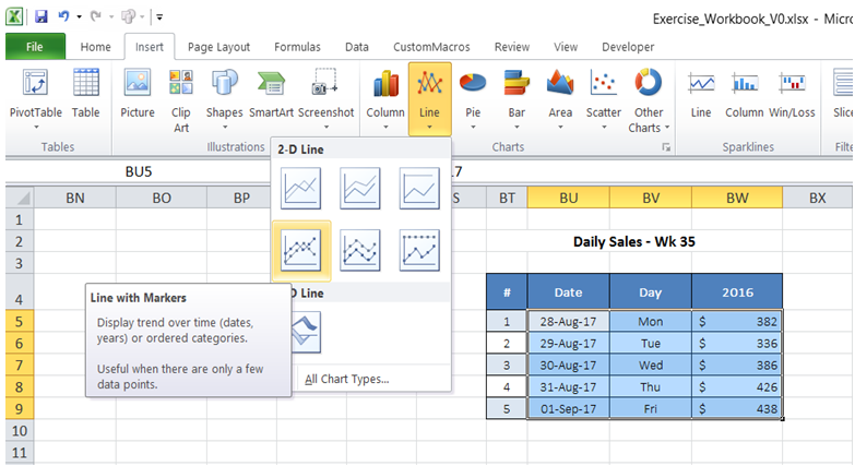
How to display text labels in the X-axis of scatter chart in ... Display text labels in X-axis of scatter chart. Actually, there is no way that can display text labels in the X-axis of scatter chart in Excel, but we can create a line chart and make it look like a scatter chart. 1. Select the data you use, and click Insert > Insert Line & Area Chart > Line with Markers to select a line chart. See screenshot: Format Chart Axis in Excel - Axis Options (Format Axis ... Right-click on the Vertical Axis of this chart and select the "Format Axis" option from the shortcut menu. This will open up the format axis pane at the right of your excel interface. Thereafter, Axis options and Text options are the two sub panes of the format axis pane. Formatting Chart Axis in Excel - Axis Options : Sub Panes
Edit titles or data labels in a chart On a chart, click the chart or axis title that you want to link to a corresponding worksheet cell. On the worksheet, click in the formula bar, and then type an equal sign (=). Select the worksheet cell that contains the data or text that you want to display in your chart. You can also type the reference to the worksheet cell in the formula bar.

Excel line chart axis labels
How to Add Axis Titles in a Microsoft Excel Chart Select the chart and go to the Chart Design tab. Click the Add Chart Element drop-down arrow, move your cursor to Axis Titles, and deselect "Primary Horizontal," "Primary Vertical," or both. In Excel on Windows, you can also click the Chart Elements icon and uncheck the box for Axis Titles to remove them both. Excel tutorial: How to create a multi level axis The goal is to create an outline that reflects what you want to see in the axis labels. Now you can see we have a multi level category axis. If I double-click the axis to open the format task pane, then check Labels under Axis Options, you can see there's a new checkbox for multi level categories axis labels. How to wrap X axis labels in a chart in Excel? And you can do as follows: 1. Double click a label cell, and put the cursor at the place where you will break the label. 2. Add a hard return or carriages with pressing the Alt + Enter keys simultaneously. 3. Add hard returns to other label cells which you want the labels wrapped in the chart axis.
Excel line chart axis labels. How-to Highlight Specific Horizontal Axis Labels in Excel ... In this video, you will learn how to highlight categories in your horizontal axis for an Excel chart. This is in answer to "I am trying to bold 5 months (ou... Change axis labels in a chart - support.microsoft.com Right-click the category labels you want to change, and click Select Data. In the Horizontal (Category) Axis Labels box, click Edit. In the Axis label range box, enter the labels you want to use, separated by commas. For example, type Quarter 1,Quarter 2,Quarter 3,Quarter 4. Change the format of text and numbers in labels How to Create Line Charts in Excel (In Easy Steps) Line charts are used to display trends over time. Use a line chart if you have text labels, dates or a few numeric labels on the horizontal axis. Use a scatter plot (XY chart) to show scientific XY data. To create a line chart, execute the following steps. 1. Select the range A1:D7. 2. On the Insert tab, in the Charts group, click the Line symbol. Add a Horizontal Line to an Excel Chart - Peltier Tech Sep 11, 2018 · The category axis of an area chart works the same as the category axis of a column or line chart, but the default settings are different. Let’s start with the following simple area chart. Notice that the first and last category labels are aligned with the corners of the plot area and the filled area series extends to the sides of the plot area.
How to change chart axis labels' font color and size in Excel? We can easily change all labels' font color and font size in X axis or Y axis in a chart. Just click to select the axis you will change all labels' font color and size in the chart, and then type a font size into the Font Size box, click the Font color button and specify a font color from the drop down list in the Font group on the Home tab. How to rotate axis labels in chart in Excel? Rotate axis labels in chart of Excel 2013 If you are using Microsoft Excel 2013, you can rotate the axis labels with following steps: 1. Go to the chart and right click its axis labels you will rotate, and select the Format Axis from the context menu. 2. Excel charts: add title, customize chart axis, legend and ... Click anywhere within your Excel chart, then click the Chart Elements button and check the Axis Titles box. If you want to display the title only for one axis, either horizontal or vertical, click the arrow next to Axis Titles and clear one of the boxes: Click the axis title box on the chart, and type the text. Skip Dates in Excel Chart Axis - myonlinetraininghub.com Jan 28, 2015 · An aside: notice how the vertical axis on the column chart starts at zero but the line chart starts at 146?That’s a visualisation rule – column charts must always start at zero because we subconsciously compare the height of the columns and so starting at anything but zero can give a misleading impression, whereas the points in the line chart are compared to the axis scale.
Excel tutorial: How to customize axis labels Instead you'll need to open up the Select Data window. Here you'll see the horizontal axis labels listed on the right. Click the edit button to access the label range. It's not obvious, but you can type arbitrary labels separated with commas in this field. So I can just enter A through F. When I click OK, the chart is updated. How to Add Axis Labels in Excel - Spreadsheeto First off, you have to click the chart and click the plus (+) icon on the upper-right side. Then, check the tickbox for 'Axis Titles'. If you would only like to add a title/label for one axis (horizontal or vertical), click the right arrow beside 'Axis Titles' and select which axis you would like to add a title/label. Editing the Axis Titles Chart Axis - Use Text Instead of Numbers - Excel & Google ... Right click Graph Select Change Chart Type 3. Click on Combo 4. Select Graph next to XY Chart 5. Select Scatterplot 6. Select Scatterplot Series 7. Click Select Data 8. Select XY Chart Series 9. Click Edit 10. Select X Value with the 0 Values and click OK. Change Labels While clicking the new series, select the + Sign in the top right of the graph How to add axis label to chart in Excel? - ExtendOffice You can insert the horizontal axis label by clicking Primary Horizontal Axis Title under the Axis Title drop down, then click Title Below Axis, and a text box will appear at the bottom of the chart, then you can edit and input your title as following screenshots shown. 4.
Text Labels on a Vertical Column Chart in Excel - Peltier Tech Blog
How To Add Axis Labels In Excel - BSUPERIOR Method 1- Add Axis Title by The Add Chart Element Option · Click on the chart area. · Go to the Design tab from the ribbon. · Click on the Add ...
31 How To Label Chart Axis In Excel - Labels For Your Ideas
Excel Chart: Horizontal Axis Labels won't update ... I created the data set in Excel 2016, selected the data and inserted a line chart. I sent one line to the secondary axis. The X axis still shows the correct labels. I sent the other line to the secondary axis and brought the first line back to the primary axis. The X axis labels are still correct. In short, I cannot reproduce the problem.
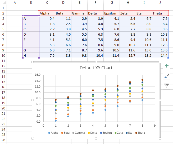
Intelligent Excel 2013 XY Charts - Peltier Tech Blog
Excel Chart not showing SOME X-axis labels - Super User Apr 05, 2017 · In Excel 2013, select the bar graph or line chart whose axis you're trying to fix. Right click on the chart, select "Format Chart Area..." from the pop up menu. A sidebar will appear on the right side of the screen. On the sidebar, click on "CHART OPTIONS" and select "Horizontal (Category) Axis" from the drop down menu.

Power BI: Dual Axis Line Chart
How to add Axis Labels (X & Y) in Excel & Google Sheets Adding Axis Labels Double Click on your Axis Select Charts & Axis Titles 3. Click on the Axis Title you want to Change (Horizontal or Vertical Axis) 4. Type in your Title Name Axis Labels Provide Clarity Once you change the title for both axes, the user will now better understand the graph.
Add Horizontal Category Axis Label Excel
How to Place Labels Directly Through Your Line Graph in ... Continue formatting a bit more. You might enlarge the label text and make that text bold so that it stands out against the gray axis labels. I often adjust the label colors so that the labels match the line (maroon numbers to match the maroon line, orange numbers to match the orange line).
Text Labels on a Vertical Column Chart in Excel - Peltier Tech Blog
Excel Chart Axis Label Tricks - My Online Training Hub Label specific Excel chart axis dates to avoid clutter and highlight specific points in time using this clever chart label trick. Jitter in Excel Scatter Charts Jitter introduces a small movement to the plotted points, making it easier to read and understand scatter plots particularly when dealing with lots of data.

Xyz graf excel | there are several different equations you need in order
Custom Axis Labels and Gridlines in an Excel Chart Jul 23, 2013 · Adding Custom Axis Labels. We will add two series, whose data labels will replace the built-in axis labels. The horizontal axis dummy series (gray line and circle markers) uses the column of numbers (E2:E8) as X values and the column of zeros (F2:F8) as Y values.
Charts in Excel - Easy Excel Tutorial
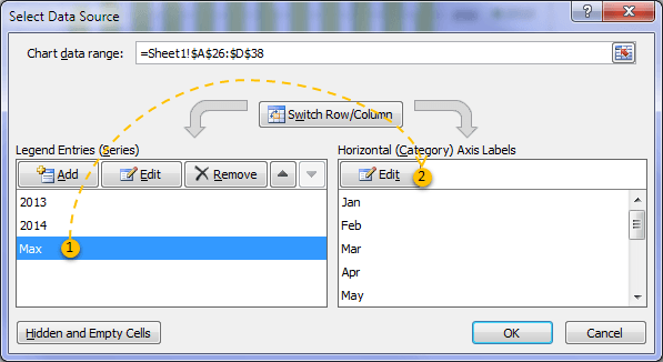
Change the display of chart axes - support.microsoft.com On the Format tab, in the Current Selection group, click the arrow in the Chart Elements box, and then click the horizontal (category) axis. On the Design tab, in the Data group, click Select Data. In the Select Data Source dialog box, under Horizontal (Categories) Axis Labels, click Edit. In the Axis label range box, do one of the following:

charts - Excel line diagram x-axis labels by week - Super User
Excel Charts: Conditionally Highlight Axis Labels on Excel ... Got a Excel Chart question? Use our FREE Excel Help. The below Excel chart highlights the X axis category labels when the monthly data drops below 25. This effect is achieved by using the data labels of 2 extra data series, plotted as lines. Here is the data and formula used to build the chart. The actual data for the column chart is in the ...

Line Chart in Excel - Easy Excel Tutorial
Dynamically Label Excel Chart Series Lines • My Online ... To modify the axis so the Year and Month labels are nested; right-click the chart > Select Data > Edit the Horizontal (category) Axis Labels > change the 'Axis label range' to include column A. Step 2: Clever Formula The Label Series Data contains a formula that only returns the value for the last row of data.
Excel Custom Chart Labels • My Online Training Hub
Label Specific Excel Chart Axis Dates - My Online Training Hub Steps to Label Specific Excel Chart Axis Dates. The trick here is to use labels for the horizontal date axis. We want these labels to sit below the zero position in the chart and we do this by adding a series to the chart with a value of zero for each date, as you can see below: Note: if your chart has negative values then set the 'Date Label ...

How-to Highlight Specific Horizontal Axis Labels in Excel Line Charts
How to Insert Axis Labels In An Excel Chart | Excelchat How to add vertical axis labels in Excel 2016/2013 We will again click on the chart to turn on the Chart Design tab We will go to Chart Design and select Add Chart Element Figure 6 - Insert axis labels in Excel In the drop-down menu, we will click on Axis Titles, and subsequently, select Primary vertical
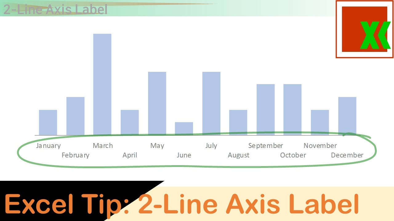
ExcelMadeEasy: Use 2 labels in x axis in charts in Excel
Change axis labels in a chart in Office In charts, axis labels are shown below the horizontal (also known as category) axis, next to the vertical (also known as value) axis, and, in a 3-D chart, next to the depth axis. The chart uses text from your source data for axis labels. To change the label, you can change the text in the source data.
How to format the chart axis labels in Excel 2010 - YouTube
Add or remove data labels in a chart On the Design tab, in the Chart Layouts group, click Add Chart Element, choose Data Labels, and then click None. Click a data label one time to select all data labels in a data series or two times to select just one data label that you want to delete, and then press DELETE. Right-click a data label, and then click Delete.

How to Change Horizontal Axis Labels in Excel 2010 - Solve Your Tech
How to stagger axis labels in Excel 21. In the chart, right click the Horizontal (Category) Axis and on the shortcut menu click Format Axis. 22. In the Format Axis pane, under Labels, set the Labels Position to None. 23. Click the Fill & Line icon and select Solid Line under Line and set the Color to Black and the Width to 1.5.
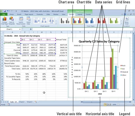
Getting to Know the Parts of an Excel 2010 Chart - dummies
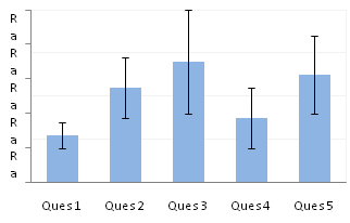
Excel Chart Vertical Axis Text Labels • My Online Training Hub Click on the top horizontal axis and delete it. Hide the left hand vertical axis: right-click the axis (or double click if you have Excel 2010/13) > Format Axis > Axis Options: Set tick marks and axis labels to None. While you're there set the Minimum to 0, the Maximum to 5, and the Major unit to 1. This is to suit the minimum/maximum values ...

Rotated axis labels in R plots | R-bloggers
How to wrap X axis labels in a chart in Excel? And you can do as follows: 1. Double click a label cell, and put the cursor at the place where you will break the label. 2. Add a hard return or carriages with pressing the Alt + Enter keys simultaneously. 3. Add hard returns to other label cells which you want the labels wrapped in the chart axis.
Post a Comment for "40 excel line chart axis labels"